Tutorial on subsets and plotting

This notebook will demostrate how to use row subsets and make plots with this package.

Updated for version 0.3.0.

Data I/O

Let’s import necessary packages and prepare our data first:

from pyttop.table import Data, Subset
import matplotlib.pyplot as plt
import numpy as np

data = Data('samples/catalog_p1.csv', name='data')
data.t

Table length=3500

x	y	z	obj_class
float64	float64	float64	str1
-4.465765915024047	-1.1803787039723304	3.933749106382124	A
-11.595113898732713	-4.049155438745423	-7.647153605424485	A
-13.658096030485229	-7.48624417464929	3.526735390303081	B
11.604269139452764	6.281875669082035	4.782030684043313	A
-0.14761531392540045	1.227243258605626	-20.026283817567307	B
14.085948012644096	13.133971787299929	34.5262446878855	B
2.2880323941946723	6.392166696793526	26.721939201307457	B
-8.154232849490825	1.271469183122783	-14.29833019843536	B
-9.120396489096619	-4.41957805036524	22.581003104515645	B
...	...	...	...
-7.5004132040390115	0.587237525937546	-3.0165053095673238	B
12.963890469507275	8.11197446790793	5.4488379845353485	A
10.522002268181685	10.457915600285398	21.314444684020117	B
-4.907849468713616	1.6191066830121663	-20.816778952996607	A
-8.39307767061386	-4.8702562712257595	2.7101045056610085	A
-24.40794608095363	-9.055720978546164	-9.880379852777681	B
8.680595630050762	5.437311273722883	20.776739109132656	A
8.619196402490193	10.131186727257958	-7.297727382124089	B
-11.657605250258602	-2.477316718617091	-49.04225493704257	B
10.045399412714959	8.895670555650621	4.670119844591375	B

data.t is an astropy.table.Table object. For more information on data input/output, see tutorial 1.

Subsets

Sometimes we need to specify row subsets of the dataset data. For example, maybe you would like to study records that satisfies both \(z>0\) and \(x>0\). The traditional method is selecting these data with indexing:

my_selected_subset = data[(data['z']>0) & (data['x']>0)]

This may be troublesome if multiple subsets (and even the intersection, union and complementary sets of them) are involved in your study.

In this package, various methods of specifying subsets are demostrated below:

Specifying subsets from selection criteria

To specify a row subset, you need to input a selection criteria (e.g. \(z>0\)), which all records in this subset should satisfy.

To define a subset of data that satisfies \(z>0\) AND \(x>0\):

subset1 = data.add_subsets(Subset((data['z']>0) & (data['x']>0), name='subset1'))

You may also directly input a string:

subset1 = data.add_subsets(Subset('(z>0) & (x>0)', name='subset1'))

[add_subsets] subset(s) at 'default/subset1' replaced

The method will try to automatically convert the string into expressions like (data.t['z']>0) & (data.t['x']>0). However, you should check the output to make sure the inferred logical expressions are correct.

One last way to specify the subset is inputting a function:

selection = lambda t: (t['z']>0) & (t['x']>0)
subset1 = data.add_subsets(Subset(selection, name='subset1'))

[add_subsets] subset(s) at 'default/subset1' replaced

The input function selection takes an astropy.table.Table object as input, and returns the boolean array (i.e. the value of expression (t['z']>0) & (t['x']>0)).

subset1 is a Subset object, which contains the information of the selection, rather than the full data table:

subset1

<Subset 'subset1' of Data 'data' (867/3500)>

To extract the dataset of this subset (\(z>0\) AND \(x>0\)), input the name ('subset1', as setted with name='subset1') to data.subset_data:

subset1_data = data.subset_data('subset1') # subset1_data is an pyttop.table.Data object
subset1_data.t

Table length=867

x	y	z	obj_class
float64	float64	float64	str1
11.604269139452764	6.281875669082035	4.782030684043313	A
14.085948012644096	13.133971787299929	34.5262446878855	B
2.2880323941946723	6.392166696793526	26.721939201307457	B
7.870877221958985	2.4497515467137005	4.8548683183511265	A
10.629256472615845	3.454185077945545	20.411033679800703	A
9.047572683607877	7.12001031357844	6.851401674467137	B
18.447207791749573	7.385454779960607	54.37398357585805	B
21.618444090858567	15.295692551348754	29.015401534486458	B
9.638420579769054	5.566364591560875	21.455050618925668	A
...	...	...	...
15.07746248914888	9.947129281184324	7.037583120882335	A
22.06034363008346	13.937223680123207	9.686905871572677	B
12.978278380713002	7.000068227499105	5.798001056268797	A
7.5708917042514665	7.099640755415276	2.6560212326271455	B
3.3172095655246867	1.0351615360304538	31.653235996934484	B
2.2271288811050094	0.003479998852875976	8.537736071994843	A
12.963890469507275	8.11197446790793	5.4488379845353485	A
10.522002268181685	10.457915600285398	21.314444684020117	B
8.680595630050762	5.437311273722883	20.776739109132656	A
10.045399412714959	8.895670555650621	4.670119844591375	B

Alternatively, you may also convert a subset1 object to a boolean array:

subset1_table = data[np.array(subset1)]
subset1_table

/tmp/ipykernel_985/1455195093.py:1: DeprecationWarning: __array__ implementation doesn't accept a copy keyword, so passing copy=False failed. __array__ must implement 'dtype' and 'copy' keyword arguments. To learn more, see the migration guide https://numpy.org/devdocs/numpy_2_0_migration_guide.html#adapting-to-changes-in-the-copy-keyword
  subset1_table = data[np.array(subset1)]

Table length=867

x	y	z	obj_class
float64	float64	float64	str1
11.604269139452764	6.281875669082035	4.782030684043313	A
14.085948012644096	13.133971787299929	34.5262446878855	B
2.2880323941946723	6.392166696793526	26.721939201307457	B
7.870877221958985	2.4497515467137005	4.8548683183511265	A
10.629256472615845	3.454185077945545	20.411033679800703	A
9.047572683607877	7.12001031357844	6.851401674467137	B
18.447207791749573	7.385454779960607	54.37398357585805	B
21.618444090858567	15.295692551348754	29.015401534486458	B
9.638420579769054	5.566364591560875	21.455050618925668	A
...	...	...	...
15.07746248914888	9.947129281184324	7.037583120882335	A
22.06034363008346	13.937223680123207	9.686905871572677	B
12.978278380713002	7.000068227499105	5.798001056268797	A
7.5708917042514665	7.099640755415276	2.6560212326271455	B
3.3172095655246867	1.0351615360304538	31.653235996934484	B
2.2271288811050094	0.003479998852875976	8.537736071994843	A
12.963890469507275	8.11197446790793	5.4488379845353485	A
10.522002268181685	10.457915600285398	21.314444684020117	B
8.680595630050762	5.437311273722883	20.776739109132656	A
10.045399412714959	8.895670555650621	4.670119844591375	B

You can also define multiple subset at a time:

subset2, subset3, subset4 = data.add_subsets(
    Subset('(x<0) | (z<0)', name='subset2'), # x<0 OR z<0
    Subset('~(y<5)', name='subset3'), # NOT (y<5)
    Subset(np.isin(data['obj_class'], ['A', 'B']), name='subset4'), # obj_class in {'A', 'B'}
    )

Convenient methods for subset definition

There are also two convenient methods to define subsets:

data.add_subsets(
    Subset.by_range(x=[0, 5], y=[0, np.inf]), # (x>0) & (x<5) & (y>0) 
    Subset.by_value('obj_class', 'A'), # obj_class == 'A'
    )

(<Subset 'x(0-5)&y(0-inf)' of Data 'data' (512/3500)>,
 <Subset 'obj_class=A' of Data 'data' (2000/3500)>)

When using the above methods, the names are automatically set (see below and help(Subset.by_range), help(Subset.by_value) for details).

Summary of subsets

Now let’s take a look at all the subsets defined so far:

data.subset_summary()

Table length=9

group	name	size	fraction	expression	label
str9	str15	int64	float64	str46	str28
$unmasked	-	-1	nan	<special subsets: item in col unmasked>	-
$eval	-	-1	nan	<special subsets: rows satisfy expression>	-
default	all	3500	1.0	all	All
default	subset1	867	0.24771428571428572	selection = lambda t: (t['z']>0) & (t['x']>0)\n	subset1
default	subset2	2633	0.7522857142857143	(x<0) | (z<0)	subset2
default	subset3	874	0.24971428571428572	~(y<5)	subset3
default	subset4	3500	1.0	<array>	subset4
default	x(0-5)&y(0-inf)	512	0.1462857142857143	(x > 0) & (x < 5) & (y > 0) & (y < inf)	x$\in$(0, 5), y$\in$(0, inf)
default	obj_class=A	2000	0.5714285714285714	obj_class=A	A

The columns of the above table are:

• group: The name of the subset group, which will be introduced in the next section.

• name: The name of the subset, which can be manully set by Subset(<...>, name=<...>).

• size: The size of this subset.

• fraction: The fraction of this subset relative to the whole dataset data.

• expression: A hint of the expression of the selection that specifies this subset. This can be manually set by Subset(<...>, expression=<...>)

• label: The string that is used for this subset in plots (e.g. label in legends and titles; see the plotting section for examples). This can be manually set by Subset(<...>, label=<...>).

We can also see that there is always a subset called “all”, which consists of all records in the dataset (that is, the whole dataset).

Now let’s clear all subsets defined above (the subset “all” is never deleted):

data.clear_subsets()
data.subset_summary() 

Table length=3

group	name	size	fraction	expression	label
str9	str3	int64	float64	str42	str3
$unmasked	-	-1	nan	<special subsets: item in col unmasked>	-
$eval	-	-1	nan	<special subsets: rows satisfy expression>	-
default	all	3500	1.0	all	All

Subset groups

This package introduces the concept of a “subset group”, which is a group of subset. This is extremely useful when you need groups of related subsets.

For example, you may want to divide the dataset according to the value of obj_class. You can define subsets in a new subset group called ‘class’:

data.add_subsets(
    Subset.by_value('obj_class', 'A'), # obj_class == 'A'
    Subset.by_value('obj_class', 'B'), # obj_class == 'B'
    group='class',
    )

(<Subset 'obj_class=A' of Data 'data' (2000/3500)>,
 <Subset 'obj_class=B' of Data 'data' (1500/3500)>)

This can be easily done with a convenient method of data:

# data.subset_group_from_values('obj_class', group_name='class') 
# -> ValueError: A subset group with name "class" already exists.
data.subset_group_from_values('obj_class', group_name='class', overwrite=True) 

Since a group named “class” already exists, we have to pass overwrite=True, though this is not necessary if group “class” has not been defined before.

In some other situations, you may want to define a group of subsets with bins of some quantity:

data.subset_group_from_ranges(
    'x', [[-20, -10], [-10, 0], [0, 10], [10, 20]], # 4 bins specified for x
    group_name='x_binning', overwrite=True, # optional arguments
    )

[<Subset 'x(-20--10)' of Data 'data' (493/3500)>,
 <Subset 'x(-10-0)' of Data 'data' (1198/3500)>,
 <Subset 'x(0-10)' of Data 'data' (1165/3500)>,
 <Subset 'x(10-20)' of Data 'data' (480/3500)>]

We can understand the outcome of the above codes by checking the subset_summary():

data.subset_summary()

Table length=9

group	name	size	fraction	expression	label
str9	str11	int64	float64	str42	str16
$unmasked	-	-1	nan	<special subsets: item in col unmasked>	-
$eval	-	-1	nan	<special subsets: rows satisfy expression>	-
default	all	3500	1.0	all	All
class	obj_class=A	2000	0.5714285714285714	obj_class=A	A
class	obj_class=B	1500	0.42857142857142855	obj_class=B	B
x_binning	x(-20--10)	493	0.14085714285714285	(x > -20) & (x < -10)	x$\in$(-20, -10)
x_binning	x(-10-0)	1198	0.3422857142857143	(x > -10) & (x < 0)	x$\in$(-10, 0)
x_binning	x(0-10)	1165	0.33285714285714285	(x > 0) & (x < 10)	x$\in$(0, 10)
x_binning	x(10-20)	480	0.13714285714285715	(x > 10) & (x < 20)	x$\in$(10, 20)

By default, if you do not specify the group name (e.g. group when calling data.add_subsets()), the group name will be “default”.

To extract the dataset of a subset in a non-default group, use one of the expressions below:

class_A_data = data.subset_data('class/obj_class=A')
class_A_data = data.subset_data(group='class', name='obj_class=A')

Making single plots

Quick reference

Note: From version 0.3.0, the previously defined plot() is unified with subplot_array() (introduced later), and it is recommended to use the new method, plots(), for most cases. However, for backward compatibility, plot() and subplot_array() can still be used.

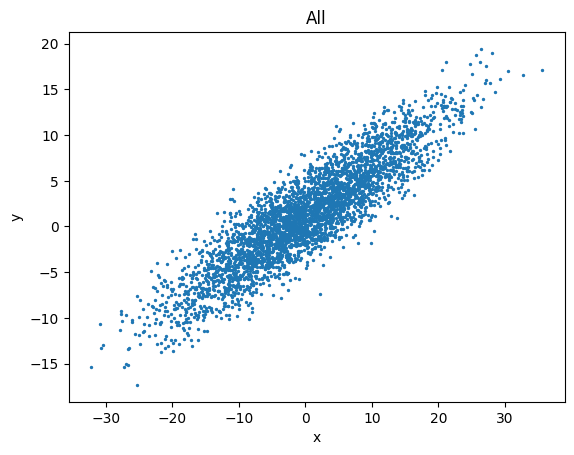
The simplest way to make a plot with pyttop.table.Data is:

data.plots('scatter', cols=['x', 'y'], s=2)
# equivalent to:
# plt.scatter(data.t['x'], data.t['y'], s=2)

(<Figure size 640x480 with 1 Axes>,
 <Axes: title={'center': 'All'}, xlabel='x', ylabel='y'>)

Where:

• 'scatter' is the type of the plot. Supported types are: 'plot', 'scatter', 'hist', 'hist2d', 'errorbar', which corresponds to plt.plot, plt.scatter, ...

• cols=['x', 'y'] specifies the column names of the dataset to be used for the plot.

• s=2 is a keyword argument passed to the plot function (in this case, plt.scatter).

To make a plot comparing different subsets in a subset group (say, 'class'):

data.plots('scatter', cols=['x', 'y'], groups='class', s=2)

(<Figure size 640x480 with 1 Axes>, <Axes: xlabel='x', ylabel='y'>)

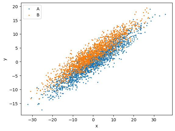
Note that in the above figure, the legend is the labels of the subsets, as shown in the output of data.subset_summary().

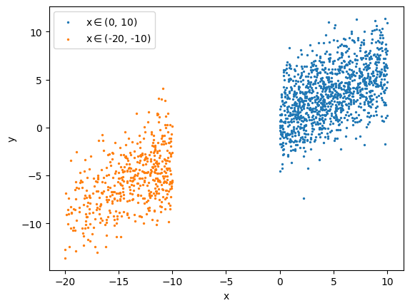
To make a plot comparing different subsets:

data.plots('scatter', cols=['x', 'y'], s=2,
          paths=['x_binning/x(0-10)', 'x_binning/x(-20--10)'],
          )

(<Figure size 640x480 with 1 Axes>, <Axes: xlabel='x', ylabel='y'>)

To make a plot with columns in the dataset as keyword arguments of the plot function:

data.plots('scatter', cols=['x', 'z'], kwcols=dict(c='y'), s=2, cmap='jet')
# equivalent to:
# s = plt.scatter(data.t['x'], data.t['z'], c=data.t['y'], s=2, cmap='jet')
# plt.colorbar(s)

(<Figure size 640x480 with 2 Axes>,
 <Axes: title={'center': 'All'}, xlabel='x', ylabel='z'>)

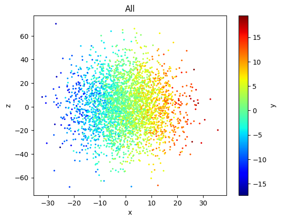
We can see that a colorbar is automatically added when color (the argument c for scatter()) is specified. To disable this, add autobar=False in the above call of data.plots(). For more information on 'scatter' plot in pyttop, see tutorials for scatter plot..

To require that all data on the plot are elements of one specific subset, provide a global selection:

data.plots('scatter', cols=['x', 'y'], groups='class', global_selection='x_binning/x(0-10)', s=4)

(<Figure size 640x480 with 1 Axes>,
 <Axes: title={'center': 'x$\\in$(0, 10)'}, xlabel='x', ylabel='y'>)

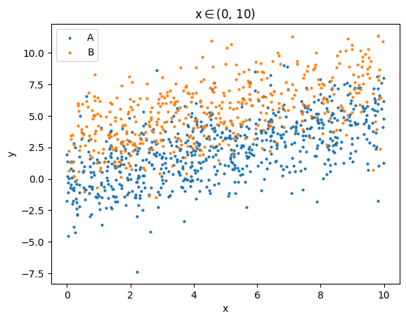
We can see that only those with \(x\in(0, 10)\) are shown on the plot. The global selection is automatically written in the title.

Advanced features

Labels of columns

By default, the labels on the axes are the column names. If you want to adjust the label of the columns, you can execute:

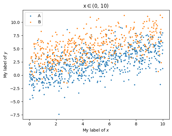
data.set_labels(x='My label of $x$', y='My label of $y$')

The setted labels can be accessed with

data.col_labels

{'x': 'My label of $x$', 'y': 'My label of $y$'}

Now the plot becomes

data.plots('scatter', cols=['x', 'y'], groups='class', global_selection='x_binning/x(0-10)', s=4)

(<Figure size 640x480 with 1 Axes>,
 <Axes: title={'center': 'x$\\in$(0, 10)'}, xlabel='My label of $x$', ylabel='My label of $y$'>)

data.col_labels = {} # clear the labels

Custom plot function

This part is for advanced users. If you are new to this package, you may skip this part for now. For more advanced use and details, see the advanced tutorial for matching and plotting.

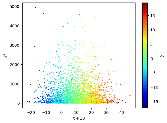
Sometimes you need more control on the plot. In general, you can input a function (rather than strings such as 'scatter') to data.plot (note: not data.plots).

fig, ax = plt.subplots(1, 1)
def my_plot(x, z, **kwargs):
    s = ax.scatter(x+10, z**2, **kwargs)
    ax.set_xlabel('$x+10$')
    ax.set_ylabel('$z^2$')
    cax = plt.colorbar(s)
    cax.set_label('$y$')
data.plot(my_plot, cols=['x', 'z'], kwcols=dict(c='y'), s=2, cmap='jet',
          autolabel=False, # we don't want to use automatically generated labels/titles this time
          )

Subplot arrays

Note: From version 0.3.0, the previously defined subplot_array() is unified with plot(), and it is recommended to use the new method, plots(), for most cases. However, for backward compatibility, plot() and subplot_array() can still be used.

Basic usage

The concept of “subplot array” is one of the hightlights of this package. To understand this concept, let’s take a look at an example first:

data.subset_group_from_ranges('x', [[-20, -10], [-10, 0], [0, 10], [10, 20]]) # the default name of the group is 'x'
data.subset_group_from_ranges('z', [[-40, 0], [0, 40]]) # the default name of the group is 'z'
data.clear_subsets('x_binning') # delete subset group 'x_binning'
data.subset_summary()

Table length=11

group	name	size	fraction	expression	label
str9	str11	int64	float64	str42	str16
$unmasked	-	-1	nan	<special subsets: item in col unmasked>	-
$eval	-	-1	nan	<special subsets: rows satisfy expression>	-
default	all	3500	1.0	all	All
class	obj_class=A	2000	0.5714285714285714	obj_class=A	A
class	obj_class=B	1500	0.42857142857142855	obj_class=B	B
x	x(-20--10)	493	0.14085714285714285	(x > -20) & (x < -10)	x$\in$(-20, -10)
x	x(-10-0)	1198	0.3422857142857143	(x > -10) & (x < 0)	x$\in$(-10, 0)
x	x(0-10)	1165	0.33285714285714285	(x > 0) & (x < 10)	x$\in$(0, 10)
x	x(10-20)	480	0.13714285714285715	(x > 10) & (x < 20)	x$\in$(10, 20)
z	z(-40-0)	1671	0.4774285714285714	(z > -40) & (z < 0)	z$\in$(-40, 0)
z	z(0-40)	1681	0.48028571428571426	(z > 0) & (z < 40)	z$\in$(0, 40)

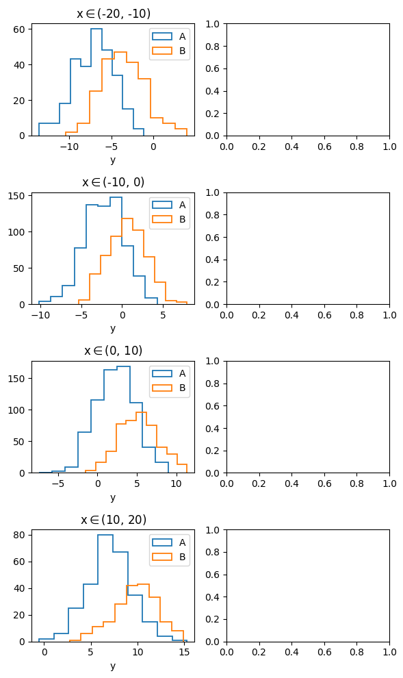
data.plots(
    'hist', cols=['y'], histtype='step', linewidth=1.3, # note: kwcols is also supported
    plotgroups='class', # subset group for comparison within each subplot
    arraygroups=['z', 'x'], # subset group for comparison between each subplot
    )
plt.tight_layout()

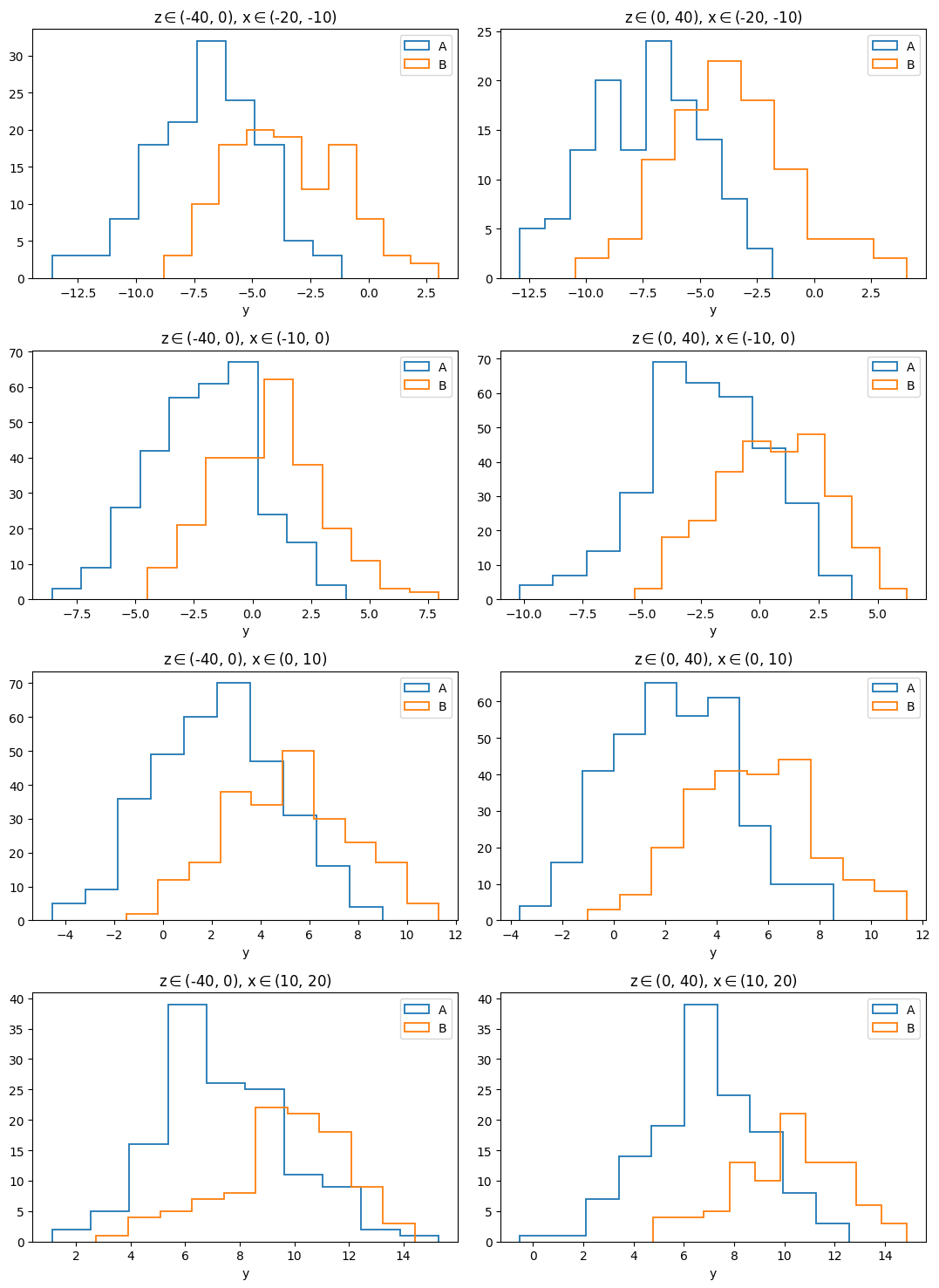
As we have seen in this example, the subset group 'x' has 4 subsets, and group 'z' has 2 subsets. By passing the argument arraygroups=['z', 'x'], the 2 subset groups are used to generate a \(4\times 2\) subplot “array”. The different rows have different selections of \(x\), while different columns have different selections of \(z\). By passing the argument plotgroups='class', the 2 subsets in the subset group named 'class' are plotted within each panel (subplot).

Sometimes you may want to generate a \(1\times n\) subplot “array”:

data.plots(
    'hist', cols=['y'], histtype='step', linewidth=1.3, # note: kwcols is also supported
    plotgroups='class', # subset group for comparison within each subplot
    arraygroups=['x'], # subset group for comparison between each subplot
    )
plt.tight_layout()

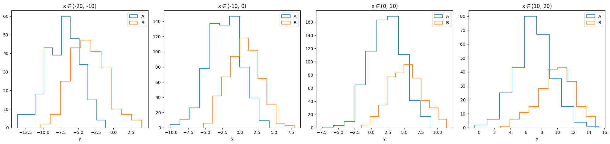
Since there are too many columns, we can try to warp this \(1\times n\) array:

data.plots(
    'hist', cols=['y'], histtype='step', linewidth=1.3, # note: kwcols is also supported
    plotgroups='class', # subset group for comparison within each subplot
    arraygroups=['x'], # subset group for comparison between each subplot
    autobreak=True, # automatically warp
    )
plt.tight_layout()

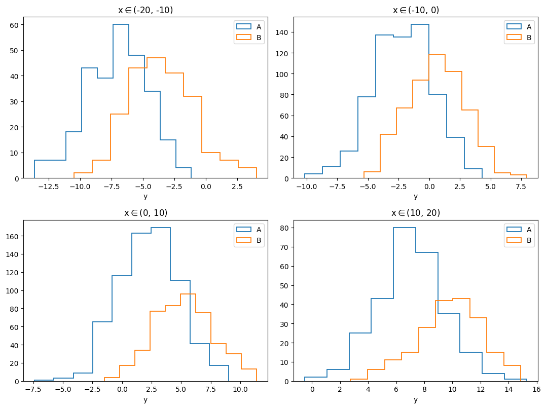
Now the \(1\times 4\) subplot array is changed into a \(2\times 2\) array.

Advanced usage

Note: This part is for advanced users. If you are new to this package, you may skip this part for now.

Callback

Sometimes you just want to do some operations on the axis of each subplot (after the plot is made):

def callback(ax): # input a axis
    ax.set_xlim(-10, 15) # set xlim for each subplot

data.plots(
    'hist', cols=['y'], histtype='step', linewidth=1.3, 
    plotgroups='class', arraygroups=['x'], autobreak=True, 
    ax_callback=callback, 
    )
plt.tight_layout()

In the above example, 2 histrograms are made for each subplot, thus the function called 'hist' is called twise for each subplot. However, the callback function is called only once for each subplot.

Custom plot function

You can also define a custom plot function, similar to that for data.plot. However, This function should input an axis (e.g. a matplotlib.axes._subplots.AxesSubplot object), and return a function that is suitable for input of data.plot.

def my_plot_func(ax): # input an axis
    def hist(*args, **kwargs):
        ax.hist(*args, **kwargs)
        ax.set_xlim(-10, 15)
    return hist

data.plots(
    my_plot_func, cols=['y'], histtype='step', linewidth=1.3, 
    plotgroups='class', arraygroups=['x'], autobreak=True, 
    )
plt.tight_layout()

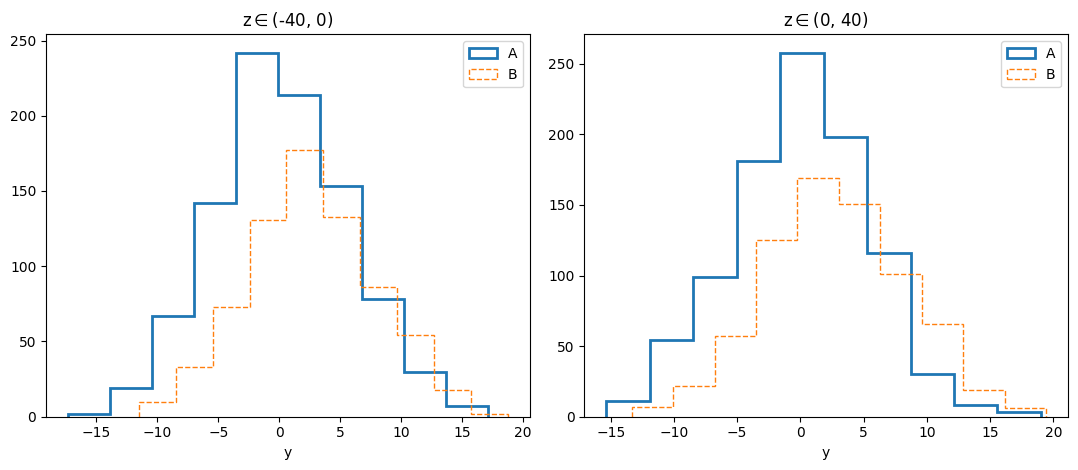
Iterative keyword arguments for plot function

If the keywoard arguments (to be passed to the plot function) are different for each subset in plotgroups, you may set them by iter_kwargs:

data.plots(
    'hist', cols=['y'], histtype='step',
    plotgroups='class', arraygroups=['z'], # group 'class' consists of two subsets, 'A' and 'B'.
    iter_kwargs={'linestyle': ['-', '--'], # kwargs for subset 'A', 'B' respectively
                 'linewidth': [2, 1]},
    )
plt.tight_layout()

Handling axes of the figure

data.subplot_array returns figure and axes of the generated figure, similar to calling fig, axes = plt.subplots(<...>).

You can also generate your figure and axes in advance, and input the axes on which you would like to make plots to data.subplot_array:

fig, axes = plt.subplots(4, 2, figsize=(6, 10))
left_panels = axes[:, 0]
fig, axes = data.plots( # data.subplot_array itself returns fig, axes
    'hist', cols=['y'], histtype='step', linewidth=1.3, 
    plotgroups='class', arraygroups=['x'], 
    axes = left_panels, # make plots on the left panels 
    )
plt.tight_layout()