A quickstart example

This tutorial demonstrates the basic steps and workflows for using PyTTOP in your project. It serves as a solid starting point and reference guide to help you understand its usage. For more detailed information, you can explore the documentation on specific topics.

Loading Data

The main class used to store tabular data in PyTTOP is Data. Let us first import it:

from pyttop.table import Data

PyTTOP includes example datasets for testing and exploring its features. Let us start by loading an example table called ‘LGM.bio’, which contains the biological properties of the fictional “little green men” (LGM).

from pyttop import get_example
lgm_bio = get_example('LGM.bio')
lgm_bio

<Data 'LGM.bio'>

Note

The “LGM” datasets are randomly generated solely for testing and demonstration purposes, with no real meaning. Please do not interpret them seriously.

As seen, the resulting lgm_bio is as Data object named ‘LGM.bio’. In most cases, you may want to load data from a file, which can be done with:

my_data = Data('path/to/data/file', name='my_data')

See the documentation here for details.

Now, we can take a look at the table we have:

lgm_bio.t

Table length=5000

id	sex	age	height	weight
int64	str7	int64	float64	float64
4982	Both	152	5.285876685178171	47.21641862351436
3638	Both	-99	4.871718461858681	49.0944637256166
3857	Female	121	5.978068021500273	59.4423357404272
2499	Female	81	3.872845897766179	36.21057288026628
1938	Female	57	4.1134717034846275	41.66593964783728
1298	Male	114	5.816001078353533	57.820407142885564
...	...	...	...	...
4176	Both	224	5.83569589806094	47.2038049736114
773	Male	79	5.13437852352276	52.56579589030932
831	Neither	51	5.469546410486544	59.79200427757866
4569	N/A	12	4.678570862408104	53.360488208662126
1000	Neither	136	4.603132905272983	40.11667243713672
4158	Female	186	7.371046528568509	71.33472061653602

Data preprocessing

It appears that the table contains some missing values, such as -99 in the ‘age’ column. To exclude these values from calculations, plots, and other analyses, we can mask them using the mask_missing() method (see here for details):

lgm_bio.mask_missing(missval=-99)

[mask missing] col 'id': 0/5000 (0.00%) masked (value: -99).
[mask missing] col 'sex': 0/5000 (0.00%) masked (value: -99).
[mask missing] col 'age': 625/5000 (12.50%) masked (value: -99).
[mask missing] col 'height': 0/5000 (0.00%) masked (value: -99).
[mask missing] col 'weight': 0/5000 (0.00%) masked (value: -99).

The output shows that 625 out of 5000 values in the ‘age’ column are missing, while the other columns do not contain -99. However, the 'N/A' entries in the ‘sex’ column also appear to represent missing values. We can mask 'N/A' specifically in the ‘sex’ column as follows:

lgm_bio.mask_missing(['sex'], missval='N/A')

[mask missing] col 'sex': 714/5000 (14.28%) masked (value: N/A).

Now let us check how the above steps take effect:

lgm_bio.t

Table masked=True length=5000

id	sex	age	height	weight
int64	str7	int64	float64	float64
4982	Both	152	5.285876685178171	47.21641862351436
3638	Both	--	4.871718461858681	49.0944637256166
3857	Female	121	5.978068021500273	59.4423357404272
2499	Female	81	3.872845897766179	36.21057288026628
1938	Female	57	4.1134717034846275	41.66593964783728
1298	Male	114	5.816001078353533	57.820407142885564
...	...	...	...	...
4176	Both	224	5.83569589806094	47.2038049736114
773	Male	79	5.13437852352276	52.56579589030932
831	Neither	51	5.469546410486544	59.79200427757866
4569	--	12	4.678570862408104	53.360488208662126
1000	Neither	136	4.603132905272983	40.11667243713672
4158	Female	186	7.371046528568509	71.33472061653602

We can make more operations on the tables, as introduced here.

Warning

This step should be done before any subset is defined (in the Defining subsets section). This is due to the static nature of susbets (see discussions here).

Matching and merging data

It is common for the information of interest to be recorded in several separate tables, such as when different properties are obtained from different surveys. Let us load more example tables about LGM:

lgm_addr = get_example('LGM.addr')
lgm_name = get_example('LGM.name')
lgm_house = get_example('LGM.house')
lgm_addr, lgm_name, lgm_house

(<Data 'LGM.addr'>, <Data 'LGM.name'>, <Data 'LGM.house'>)

'LGM.addr' contains the addresses, described by longitude called 'ra' and latitude called 'dec':

lgm_addr.t

Table length=5000

id	ra	dec
int64	float64	float64
4982	136.0854386410856	86.1501075643242
3638	90.45487825432775	26.68961090066547
3857	327.2846655844139	-35.76782461457626
2499	357.1661362826631	59.75263306402611
1938	258.0935565368864	43.62751110462609
1298	288.1021019923507	-18.0319889117823
...	...	...
4176	351.4056404985322	5.242588496591069
773	172.39697961657959	-13.027380226082531
831	44.46225264213912	-64.93410115013465
4569	140.74582101419014	11.24210612306192
1000	101.24854807472687	3.9419081639703397
4158	129.306401715813	23.739275822120526

'LGM.name' contains the names of LGM:

lgm_name.t

Table length=3500

id	surname
int64	str10
2885	Patterson
1885	Sanchez
2814	Parker
3571	Bryant
1537	Jackson
2006	Wright
...	...
1353	Stewart
835	Washington
4117	Knight
3638	Parker
1168	Perkins
29	Scott

and 'LGM.house' contains information about the houses at each location:

lgm_house.t

Table length=5000

ra	dec	area
float64	float64	float64
136.0854386410856	86.1501075643242	30.12559414147148
90.45487825432775	26.68961090066547	22.588093897628738
327.2846655844139	-35.76782461457626	24.700022953216845
357.1661362826631	59.75263306402611	26.007538891355942
258.0935565368864	43.62751110462609	24.77640003628158
288.1021019923507	-18.0319889117823	21.509310818316457
...	...	...
351.4056404985322	5.242588496591069	19.203126237682365
172.39697961657959	-13.027380226082531	22.044461226220715
44.46225264213912	-64.93410115013465	26.968278557675564
140.74582101419014	11.24210612306192	23.402062063352645
101.24854807472687	3.9419081639703397	18.977101898408353
129.306401715813	23.739275822120526	22.908667591094602

To analyze our data, we may need to match rows that represent the same instance and merge all the table mentioned above (lgm_bio, lgm_addr, lgm_name, lgm_house). To match tables, we first need to import the appropriate “matchers”:

from pyttop.matcher import ExactMatcher, SkyMatcher

Note that lgm_bio, lgm_addr, and lgm_name all contain the “id” column, so we can use the ExactMatcherto match rows where the “id” values are exactly the same.

lgm_bio.match(lgm_name, ExactMatcher('id', 'id')) # `'id', 'id'` are colmun names for `lgm_bio` and `lgm_name`, respectively.
lgm_bio.match(lgm_addr, ExactMatcher('id')); # if the two column names are the same

[match] "LGM.name" matched to "LGM.bio": 3500/5000 matched.
[match] "LGM.addr" matched to "LGM.bio": 5000/5000 matched.

As shown in the output, all 5000 rows in "lGM.bio" have matching rows in "LGM.addr", but only 3500 of them have matches in "LGM.name". In other words, 1500 “id” values in "lGM.bio" do not have corresponding entries in "LGM.name".

To merge the "LGM.house" table, we can match it with "LGM.addr" based on the longitude and latitude coordinates (ra, dec), using SkyMatcher, since the "LGM.house" table does not contain the “id” column.

lgm_addr.match(lgm_house, SkyMatcher());

[SkyMatcher] Data LGM.addr: found RA name 'ra' and Dec name 'dec'.
[SkyMatcher] Data LGM.house: found RA name 'ra' and Dec name 'dec'.

[match] "LGM.house" matched to "LGM.addr": 5000/5000 matched.

In this case, the ‘ra’ and ‘dec’ columns are automatically detected. Since (ra, dec) may contain errors, entries with the closest positions and distances smaller than a threshold (defaulting to 1 arcsec) are matched. We can also explicitly specify the RA and Dec column names and the threshold thres:

lgm_house.match(lgm_addr, SkyMatcher(thres=1, coord='ra-dec', coord1='ra-dec'));

[match] "LGM.addr" matched to "LGM.house": 5000/5000 matched.

Caution

In astronomy, RA can be expressed in hours. If the RA column does not have units (e.g. data.t['RA'].unit), SkyMatcher assumes the values are in degrees. You may need to specify the units as described here. Failing to do so can lead to incorrect matching results, which may not be immediately apparent.

Tip

By matching using data.match(data1, <...>), we try to find one best matching row (if any) in data1 for each row in data. This implies differences between lgm_addr.match(lgm_house, <...>) and lgm_house.match(lgm_addr, <...>)when , e.g., some instances are included in one table but not in the other table. For more details, see the matching documentation.

For simplicity, we will refer to data.match(data1, <...>) as “data1 matched to data”.

We can check how tables are matched to "lGM.bio", either directly or through intermediate tables, using the match_tree() method:

lgm_bio.match_tree()

Names with parentheses are already matched, thus they are not expanded and will be ignored when merging.
---------------
LGM.bio [base]
:   LGM.name [ExactMatcher("id", "id")]
:   LGM.addr [ExactMatcher("id", "id")]
:   :   LGM.house [<SkyMatcher with thres=1>]
:   :   :   (LGM.addr) [<SkyMatcher with thres=1>]
---------------

As shown, two datasets, "LGM.name" and "LGM.addr", are matched directly to our base data, "lGM.bio", using the ExactMatcher. "LGM.house" is matched to "LGM.addr" and can thus be merged as well. Although "LGM.addr" is also matched to "LGM.house", since we already have "LGM.addr", we do not need to count it again.

We can now merge all these tables using the merge() method:

lgm = lgm_bio.merge() # `lgm` is the merged dataset
lgm.t

Names with parentheses are already matched, thus they are not expanded and will be ignored when merging.
---------------
LGM.bio
:   LGM.name
:   LGM.addr
:   :   LGM.house
:   :   :   (LGM.addr)
---------------

[merge] merged: LGM.bio, LGM.name, LGM.addr, LGM.house

Table length=3500

id_LGM.bio	sex	age	height	weight	id_LGM.name	surname	id_LGM.addr	ra_LGM.addr	dec_LGM.addr	ra_LGM.house	dec_LGM.house	area
int64	str7	int64	float64	float64	int64	str10	int64	float64	float64	float64	float64	float64
4982	Both	152	5.285876685178171	47.21641862351436	4982	Johnston	4982	136.0854386410856	86.1501075643242	136.0854386410856	86.1501075643242	30.12559414147148
3638	Both	--	4.871718461858681	49.0944637256166	3638	Parker	3638	90.45487825432775	26.68961090066547	90.45487825432775	26.68961090066547	22.588093897628738
2499	Female	81	3.872845897766179	36.21057288026628	2499	Hughes	2499	357.1661362826631	59.75263306402611	357.1661362826631	59.75263306402611	26.007538891355942
1938	Female	57	4.1134717034846275	41.66593964783728	1938	Richardson	1938	258.0935565368864	43.62751110462609	258.0935565368864	43.62751110462609	24.77640003628158
1298	Male	114	5.816001078353533	57.820407142885564	1298	Adams	1298	288.1021019923507	-18.0319889117823	288.1021019923507	-18.0319889117823	21.509310818316457
2788	--	160	4.940093837899926	42.131509571914805	2788	Simmons	2788	184.6162228323339	28.355354989748907	184.6162228323339	28.355354989748907	22.782082185683507
...	...	...	...	...	...	...	...	...	...	...	...	...
4366	Neither	--	5.740004480141956	66.01787750568623	4366	Alvarez	4366	2.843122795075148	67.18538172339406	2.843122795075148	67.18538172339406	27.44336793418737
773	Male	79	5.13437852352276	52.56579589030932	773	Knight	773	172.39697961657959	-13.027380226082531	172.39697961657959	-13.027380226082531	22.044461226220715
831	Neither	51	5.469546410486544	59.79200427757866	831	Cameron	831	44.46225264213912	-64.93410115013465	44.46225264213912	-64.93410115013465	26.968278557675564
4569	--	12	4.678570862408104	53.360488208662126	4569	Cameron	4569	140.74582101419014	11.24210612306192	140.74582101419014	11.24210612306192	23.402062063352645
1000	Neither	136	4.603132905272983	40.11667243713672	1000	Knight	1000	101.24854807472687	3.9419081639703397	101.24854807472687	3.9419081639703397	18.977101898408353
4158	Female	186	7.371046528568509	71.33472061653602	4158	Cooper	4158	129.306401715813	23.739275822120526	129.306401715813	23.739275822120526	22.908667591094602

The resulting table includes only 3500 rows, as only 3500 out of 5000 were matched when matching "LGM.name" to "LGM.bio". However, we may want to retain rows without "LGM.name" information. Also, the resulting table appears redundant as, e.g., it includes the “id” column from three datasets: 'id_LGM.bio', 'id_LGM.name', and 'id_LGM.addr'. We can control which columns should be ignored or merged. To achieve this, we can make some adjustments to the code:

lgm = lgm_bio.merge(
    keep_unmatched=['LGM.name'], # set it to True to keep unmatched rows for all tables
    merge_columns={
        'LGM.name': ['surname'], # only merges this column
    },
    ignore_columns={
        'LGM.addr': ['id'],
        'LGM.house': ['ra', 'dec'], # do not merge these columns
    },
)
lgm.t

Names with parentheses are already matched, thus they are not expanded and will be ignored when merging.
---------------
LGM.bio
:   LGM.name
:   LGM.addr
:   :   LGM.house
:   :   :   (LGM.addr)
---------------
[merge] entries with no match for LGM.name is kept.
[merge] merged: LGM.bio, LGM.name, LGM.addr, LGM.house

Table length=5000

id	sex	age	height	weight	surname	ra	dec	area
int64	str7	int64	float64	float64	str10	float64	float64	float64
4982	Both	152	5.285876685178171	47.21641862351436	Johnston	136.0854386410856	86.1501075643242	30.12559414147148
3638	Both	--	4.871718461858681	49.0944637256166	Parker	90.45487825432775	26.68961090066547	22.588093897628738
3857	Female	121	5.978068021500273	59.4423357404272	--	327.2846655844139	-35.76782461457626	24.700022953216845
2499	Female	81	3.872845897766179	36.21057288026628	Hughes	357.1661362826631	59.75263306402611	26.007538891355942
1938	Female	57	4.1134717034846275	41.66593964783728	Richardson	258.0935565368864	43.62751110462609	24.77640003628158
1298	Male	114	5.816001078353533	57.820407142885564	Adams	288.1021019923507	-18.0319889117823	21.509310818316457
...	...	...	...	...	...	...	...	...
4176	Both	224	5.83569589806094	47.2038049736114	--	351.4056404985322	5.242588496591069	19.203126237682365
773	Male	79	5.13437852352276	52.56579589030932	Knight	172.39697961657959	-13.027380226082531	22.044461226220715
831	Neither	51	5.469546410486544	59.79200427757866	Cameron	44.46225264213912	-64.93410115013465	26.968278557675564
4569	--	12	4.678570862408104	53.360488208662126	Cameron	140.74582101419014	11.24210612306192	23.402062063352645
1000	Neither	136	4.603132905272983	40.11667243713672	Knight	101.24854807472687	3.9419081639703397	18.977101898408353
4158	Female	186	7.371046528568509	71.33472061653602	Cooper	129.306401715813	23.739275822120526	22.908667591094602

As seen, those without match for “surname” are masked.

Now with our combined dataset, we are ready to analyze it.

Defining subsets

It is common to be interested in subsets of a dataset. For example, we might want to know how many of the “little green men” have the surname “Smith”. So let us import Subset and add a subset:

from pyttop.table import Subset

smith = lgm.add_subsets(
    Subset.by_value('surname', 'Smith'), # Defines a subset for rows where the 'surname' column is 'Smith'
    )
smith

<Subset 'surname=Smith' of Data '(LGM.bio).MATCH(LGM.name, LGM.addr, LGM.house)' (47/5000)>

As shown in the output, 47 out of 5000 entries have the surname “Smith”.

We may also want to study potential systematic differences between sexes. To do so, let us create a “subset group” for the different sexes:

lgm.subset_group_from_values('sex')
lgm.get_subsets(name=['sex=Male', 'sex=Female'])

[subset] Found subset 'sex=Male' in group 'sex'.
[subset] Found subset 'sex=Female' in group 'sex'.

[<Subset 'sex=Male' of Data '(LGM.bio).MATCH(LGM.name, LGM.addr, LGM.house)' (1036/5000)>,
 <Subset 'sex=Female' of Data '(LGM.bio).MATCH(LGM.name, LGM.addr, LGM.house)' (1031/5000)>]

Here are all subsets we have:

lgm.subset_summary()

Table length=8

group	name	size	fraction	expression	label
str9	str13	int64	float64	str42	str7
$unmasked	-	-1	nan	<special subsets: item in col unmasked>	-
$eval	-	-1	nan	<special subsets: rows satisfy expression>	-
default	all	5000	1.0	all	All
default	surname=Smith	47	0.0094	surname=Smith	Smith
sex	sex=Both	1096	0.2192	sex=Both	Both
sex	sex=Female	1031	0.2062	sex=Female	Female
sex	sex=Male	1036	0.2072	sex=Male	Male
sex	sex=Neither	1123	0.2246	sex=Neither	Neither

There are more ways to define and use subsets. See the subset documentation for details.

Making plots

To quicky explore the patterns in our data, it is a good idea to create some plots.

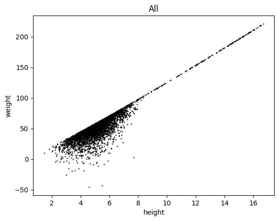
Let us begin by plotting weight versus height for all entries:

lgm.scatter('height', 'weight', c='k', s=.5, subsets='all')

(<Figure size 640x480 with 1 Axes>,
 <Axes: title={'center': 'All'}, xlabel='height', ylabel='weight'>)

Is there any differences between sexes?

lgm.scatter('height', 'weight', s=.5, 
    group='sex',
    )

(<Figure size 640x480 with 1 Axes>, <Axes: xlabel='height', ylabel='weight'>)

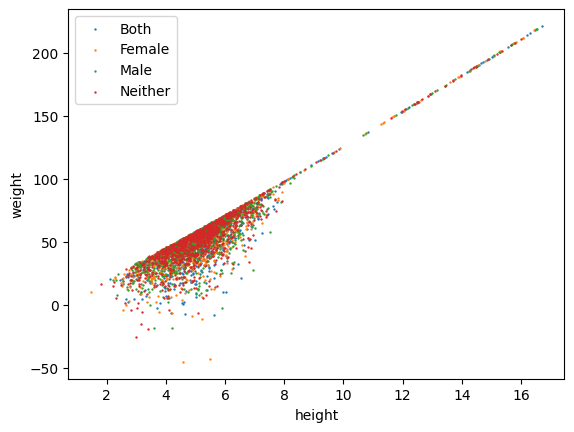
It seems there is no sexual dependance for height and weight. Then, can there be a dependance on age? We can color-code the markers by age:

lgm.scatter('height', 'weight', s=.5, c='age', cmap='jet', subsets='all')

(<Figure size 640x480 with 2 Axes>,
 <Axes: title={'center': 'All'}, xlabel='height', ylabel='weight'>)

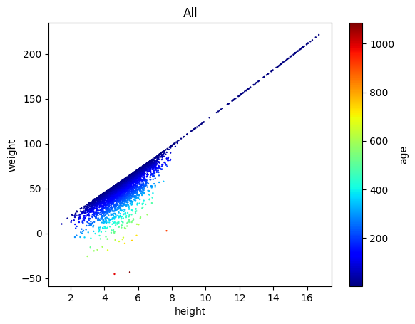
Great, so their weight at a given height is determined by the age. By the way, we can change lgm.scatter() to lgm.plots() for more general usage (see here for details):

lgm.plots(
    'scatter', # making a scatter plot
    cols=('height', 'weight'), # column 'weight' versus 'height'
    kwcols={'c': 'age'}, # color-coding: column 'age'
    s=.5, cmap='jet', # more scatter settings
    subsets='all', # plotting all rows
    )

(<Figure size 640x480 with 2 Axes>,
 <Axes: title={'center': 'All'}, xlabel='height', ylabel='weight'>)

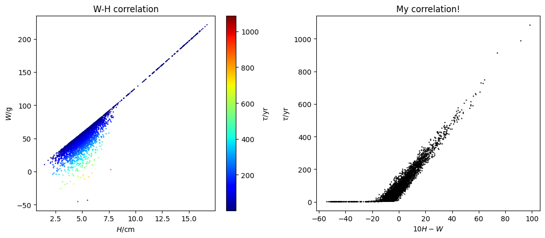
It seems that the dependence on age can be better shown by the following correlation:

lgm.plots(
    'scatter', # making a scatter plot
    cols=('10*height - weight', 'age'), # 'age' versus 'weight - 10**height' 
    eval=True, # we need to evaluate the above expression (since '10*height - weight' is not a column name)
    s=.5, # more scatter settings
    subsets='all', # plotting all rows
    )

(<Figure size 640x480 with 1 Axes>,
 <Axes: title={'center': 'All'}, xlabel='10*height - weight', ylabel='age'>)

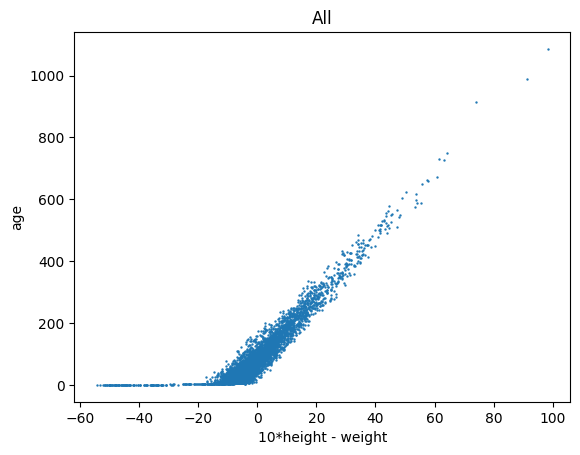
This appears to be a good correlation. So let us define a new quantity \(q\): \( q = W - 10H, \) where \(W\) denotes weight and \(H\) denotes height. We can calculate this and add it as a new column (see here for details):

lgm.eval('10*height - weight', to_col='q'); # evaluate '10*height - weight' and store it in the column 'q'

Great, let us report this in our new paper, On the Properties of the Little Green Men. However, we might want to set the labels more formally, rather than directly showing column names (see here for details):

lgm.set_labels(
    height=r'$H/\mathrm{cm}$',
    weight=r'$W/\mathrm{g}$',
    age=r'$\tau/\mathrm{yr}$',
    )

Now, with more control, we can further customize the plots (see here for details):

import matplotlib.pyplot as plt
fig, axes = plt.subplots(1, 2, figsize=(10.8, 4.8))

lgm.plots(
    'scatter', # making a scatter plot
    cols=('height', 'weight'), # column 'weight' versus 'height'
    kwcols={'c': 'age'}, # color-coding: column 'age'
    s=.5, cmap='jet', # more scatter settings
    subsets='all', # plotting all entries
    ax=axes[0], # plot it in the first axis
    )
lgm.plots(
    'scatter', # making a scatter plot
    cols=('10*height - weight', 'age'), # 'age' versus 'weight - 10**height' 
    eval=True, # we need to evaluate the above expression ('10*height - weight' is not a column name)
    s=.5, c='k', # more scatter settings
    subsets='all', # plotting all entries
    ax=axes[1], # plot it in the second axis
    )

# manual adjustments
axes[0].set_title('W-H correlation')
axes[1].set_title('My correlation!')
axes[1].set_xlabel('$10H-W$')
plt.tight_layout()

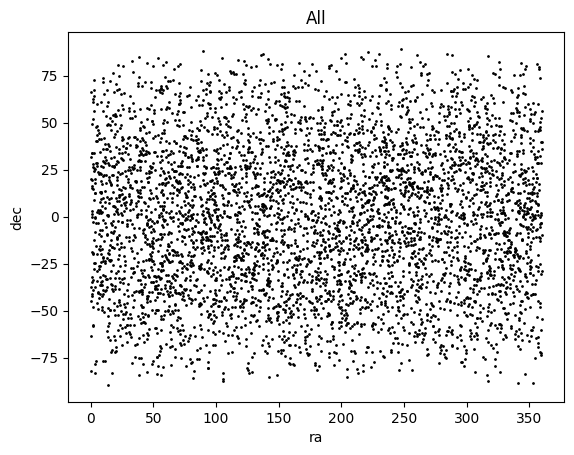
As another example, let us study the house information of the LGMs.

lgm.plots(
    'scatter',
    cols=('ra', 'dec'),
    s=1, c='k',
    subsets='all',
    )

(<Figure size 640x480 with 1 Axes>,
 <Axes: title={'center': 'All'}, xlabel='ra', ylabel='dec'>)

Suppose we are interested in the locations where LGMs with the surname “Smith” live:

lgm.plots(
    'scatter',
    cols=('ra', 'dec'),
    subsets=(~smith, smith), # `smith` is a subset defined eariler; `~smith` is its complementary set (not in `smith`)
    iter_kwargs={ # for the two subsets, `~smith` and `smith`, use two different settings
        's': [.5, 5],
        'c': ['gray', 'r'],
        'marker': ['.', '*'],
        },
    )

(<Figure size 640x480 with 1 Axes>, <Axes: xlabel='ra', ylabel='dec'>)

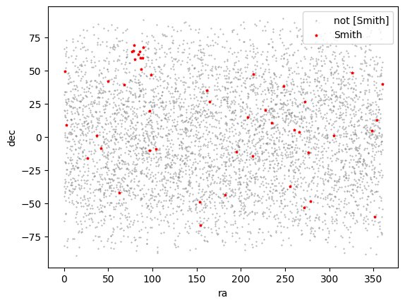
There appears to be a group of LGMs with the surname “Smith” living around ra = 80, dec = 60.

There are many more features of the plots() method. Check the documentation for details.

Saving and exporting data

Now, we would like to save our merged dataset for later use. With the following code, we can save it to the lgm.data file, which can be loaded later by PyTTOP (see here for details).

# lgm.save('path/to/lgm.data')

To publish or share our dataset, we may also need to export it using a certain format (see here for more information):

# lgm.save('path/to/lgm.txt', format='ascii')