Making Plots Given Subsets

It is common to plot only a subset of a dataset (e.g., when only some rows have good data quality) or to compare plots of several subsets (e.g., when comparing different populations). This page explains how to plot a single subset or multiple subsets, as well as how to plot different subsets on different axes.

For demonstration, an example dataset will be used:

from pyttop import get_example
from pyttop.table import Data, Subset
import matplotlib.pyplot as plt

data = get_example('P1')
data.t

Table length=3500

x	y	z	m	obj_class
float64	float64	float64	float64	str1
0.3461187418525562	0.108110723091368	6.791852465103682	1.4332289403413219	A
0.08367253256452209	-0.24948418116634086	18.951791348290804	29.1136245309425	B
3.93376870254097	1.1505379992925766	22.737372669011265	3.6996866294608246	A
-5.31142208357589	-1.484606174965062	-0.773043567821706	23.552214159958623	B
...	...	...	...	...
-4.083331628266692	-0.5630137627835397	26.0946339964304	-4.170702898759859	A
-11.785970500010595	0.73552451669164	-6.002479735924865	16.647842729068927	B
-4.841694333335785	1.1357946467717523	-2.6615288402253383	-4.633028434371802	A
-0.1293876810358806	-0.2095185181790277	12.423951189058046	0.3236923936518824	A

Some subsets will be defined for demonstration (see the documentation for subsets for explanations of the methods used in the code below):

data.subset_group_from_values('obj_class', group_name='class')
data.subset_group_from_ranges(
    'x', [[-20, -10], [-10, 0], [0, 10], [10, 20]], # 4 bins specified for x
    group_name='x_bins',
    )
data.subset_group_from_ranges(
    'z', [[-40, 0], [0, 40]],
    group_name='z_bins',
    )
subset_A = data.get_subsets(name='obj_class=A')
subset_xbin = data.get_subsets('x_bins/x(0-10)')
data.subset_summary()

[subset] Found subset 'obj_class=A' in group 'class'.

Table length=11

group	name	size	fraction	expression	label
str9	str11	int64	float64	str42	str16
$unmasked	-	-1	nan	<special subsets: item in col unmasked>	-
$eval	-	-1	nan	<special subsets: rows satisfy expression>	-
default	all	3500	1.0	all	All
class	obj_class=A	2000	0.5714285714285714	obj_class=A	A
...	...	...	...	...	...
x_bins	x(0-10)	1193	0.34085714285714286	(x > 0) & (x < 10)	x$\in$(0, 10)
x_bins	x(10-20)	449	0.12828571428571428	(x > 10) & (x < 20)	x$\in$(10, 20)
z_bins	z(-40-0)	1679	0.4797142857142857	(z > -40) & (z < 0)	z$\in$(-40, 0)
z_bins	z(0-40)	1669	0.47685714285714287	(z > 0) & (z < 40)	z$\in$(0, 40)

In a single axis

Given one or several subsets

You can specify a single or several subsets to plot using the group, subsets, or paths arguments, which correspond to the group, name, and path arguments in the get_subsets() method, as describied here. Below are several usage examples:

data.plots(
    'scatter', 
    cols=('x', 'y'), kwcols={'c': 'z'},
    s=2,
    subsets='obj_class=B',
    );

[subset] Found subset 'obj_class=B' in group 'class'.

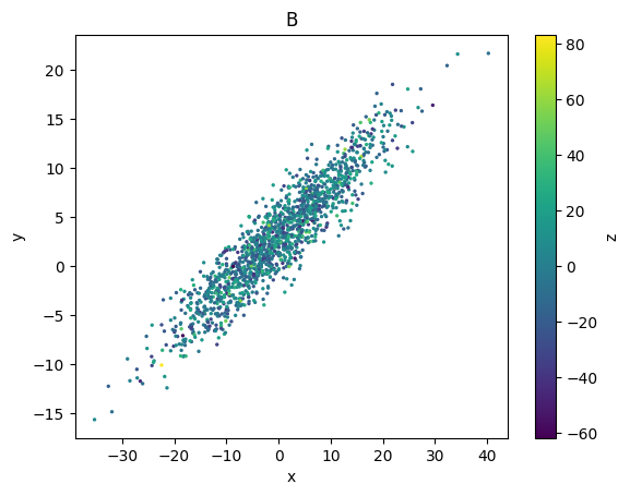
In the above code, a single subset is specified by its name using the subsets argument. The subset label ('B') is automatically shown in the axis title.

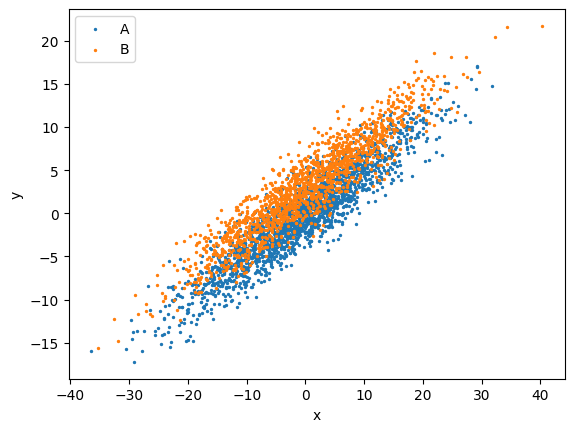
data.plots(
    'scatter', 
    cols=('x', 'y'), 
    s=2,
    paths=['class/obj_class=A', 'x_bins/x(10-20)'],
    );

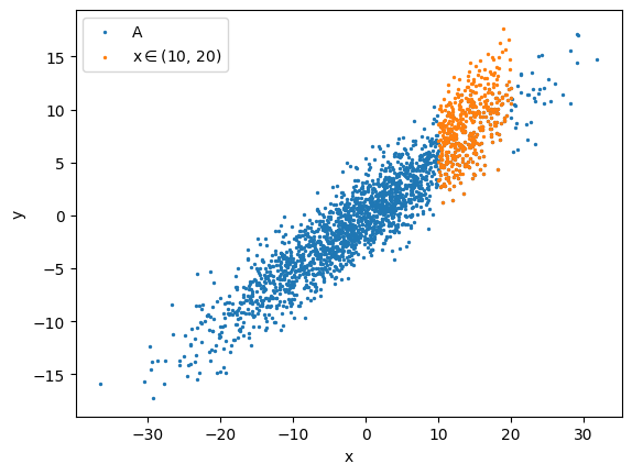
In the above code, two subsets are specified using the paths argument. In this case, the subset labels are automatically included in the legend.

The paths also accepts special subsets:

data.plots(
    'scatter', 
    cols=('x', 'y'), 
    s=2,
    paths=['$eval:obj_class=="A"', '$eval:(10 < x) & (x < 20)'],
    );

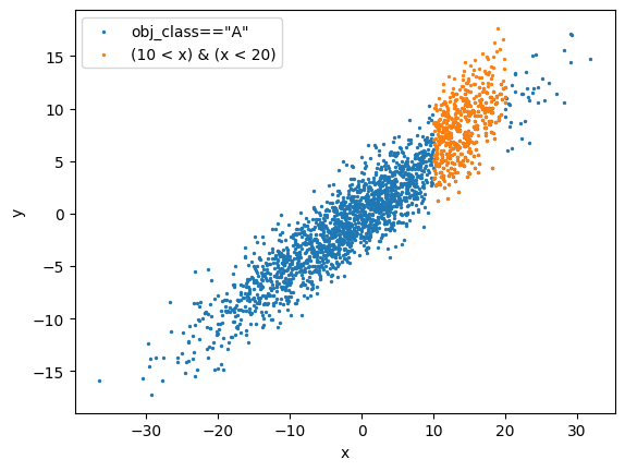
This can be used to quickly explore the data without explicitly defining the subsets.

Both paths and subsets accepts Subset objects. For example:

print(subset_A, subset_xbin, subset_A & subset_xbin)
data.plots(
    'scatter', 
    cols=('x', 'y'), kwcols={'c': 'z'},
    s=2,
    subsets=subset_A & subset_xbin,
    );

<Subset 'obj_class=A' of Data 'P1' (2000/3500)> <Subset 'x(0-10)' of Data 'P1' (1193/3500)> <Subset 'obj_class=A AND x(0-10)' of Data 'P1' (701/3500)>

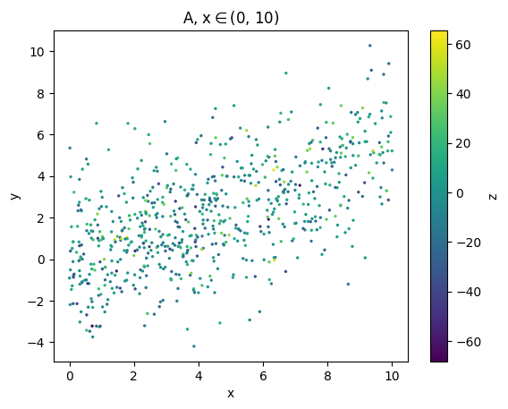
As shown, the intersection set of the two subsets is specified, and the resulting subset label (shown in the title) is automatically generated.

Given a subset group

One can also specify a subset group instead of individual subsets:

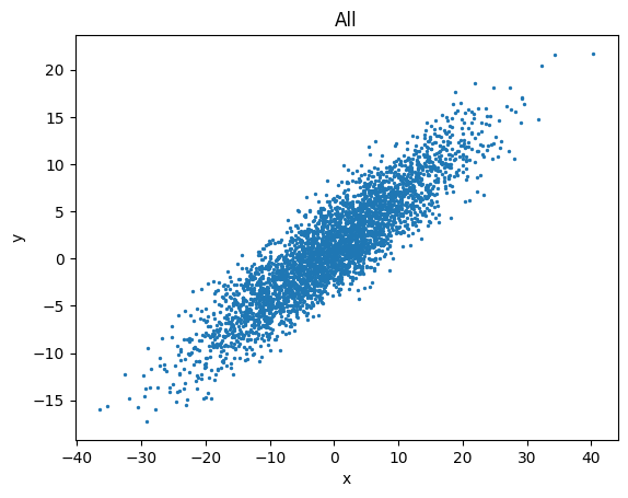
data.plots(
    'scatter', 
    cols=('x', 'y'), 
    s=2,
    group='class',
    );

In the above code, a subset group is specifed, so all subsets within the given group are plotted.

By default, plots() plots all subsets in the 'default' group, which includes one subset (named 'all') containing all rows if no other subsets are added to the 'default' group.

data.plots(
    'scatter', 
    cols=('x', 'y'), 
    s=2,
    # group='default',
    );

In multiple axes (subplots)

Given a subset group

To compare different subsets by plotting them in various axes (subplots), set the arraygroups argument to the group name:

data.plots(
    'hist', cols='y',
    arraygroups='x_bins',
    );

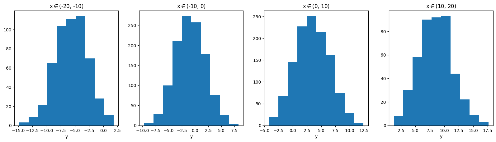
As shown, each subplot displays the data for a specific subset, with the subset label included in the titles.

Given several subset groups

You can also specify two subset groups for arraygroups, which will result in an array of subplots:

data.plots(
    'hist', cols='y',
    arraygroups=('x_bins', 'z_bins'),
    )
plt.tight_layout()

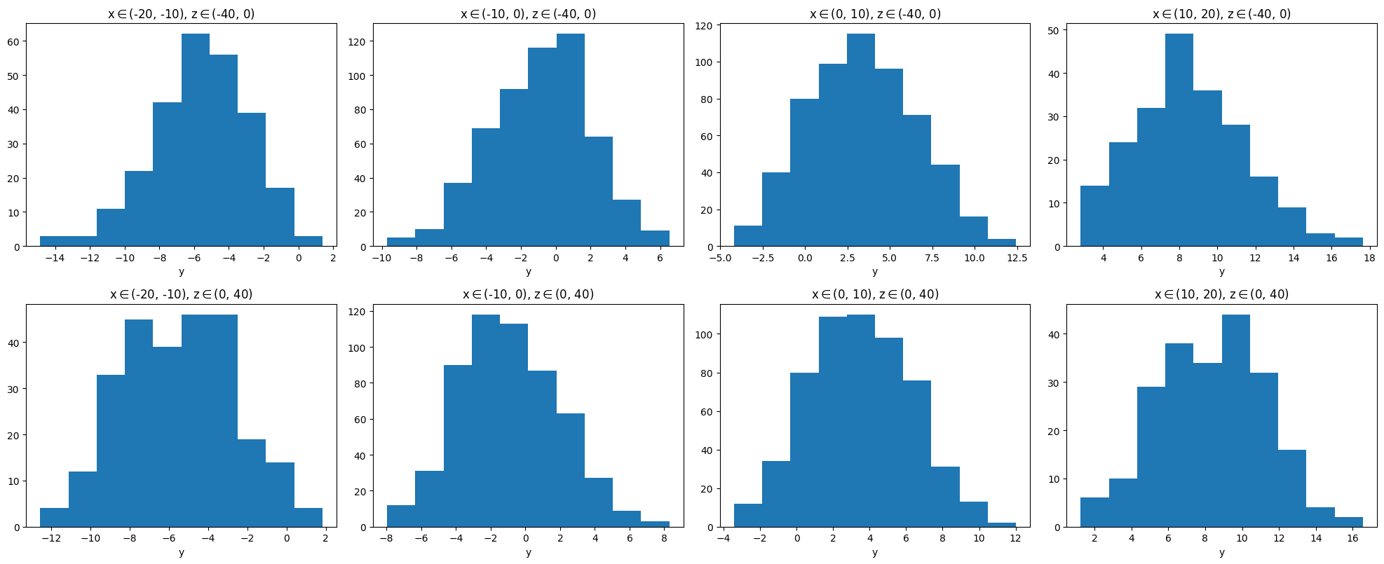
For example, the upper left panel plots the data that satisfies both \(-20 < x < -10\) and \(-40 < z < 0\).

The arraygroups can be combined with the aformentioned methods to overplot subsets:

data.plots(
    'hist', cols='y',
    plotgroups='class', # `plotgroups` is an alternative to the `group` argument
    arraygroups=('x_bins', 'z_bins'),
    )
plt.tight_layout()

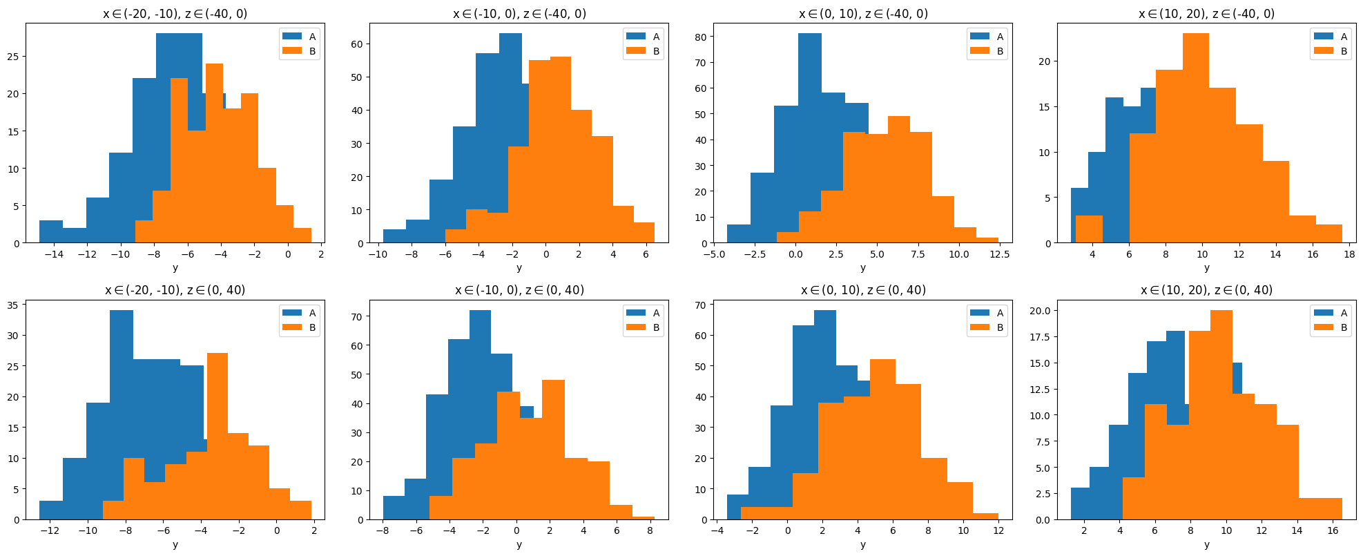
In this example, the data in each panel is further separated into the two classes, 'A' and 'B'.

Miscellaneous

Global selection

You can set the global_selection argument to a subset or its path so that only rows within the specified subset are plotted. You can also provide a list of subsets, in which case the intersection set of these subsets will be used.

data.plots(
    'hist', cols='y',
    arraygroups=('x_bins', 'z_bins'),
    global_selection=subset_A, 
    # some other valid examples: 
    # global_selection='class/obj_class=A', 
    # global_selection=['class/obj_class=A', 'x_bins/x(0-10)'], # the intersection set of them
    )
plt.tight_layout()

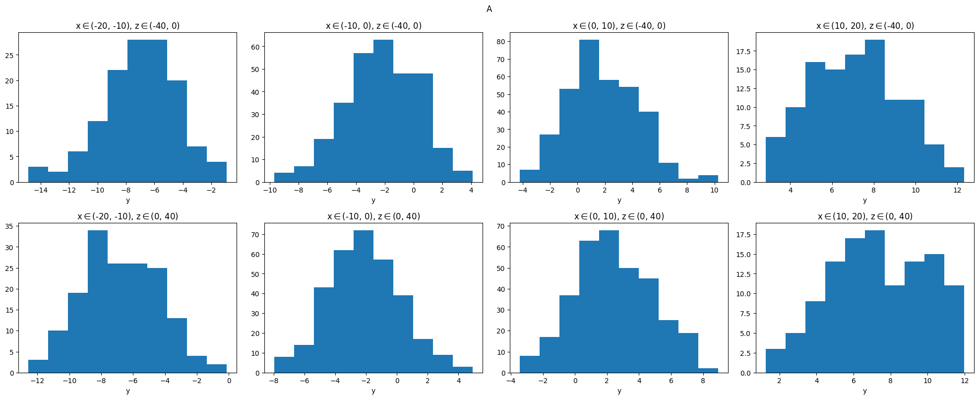
As seen in the example above, the global selection is indicated in the topmost title (suptitle in matplotlib).

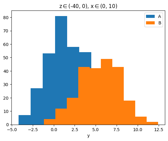
The global selection will be automatically indicated in a reasonable manner, as shown in the examples below:

data.plots(
    'hist', cols='y',
    group='class',
    global_selection=['z_bins/z(-40-0)', 'x_bins/x(0-10)'], # the intersection of them
    );

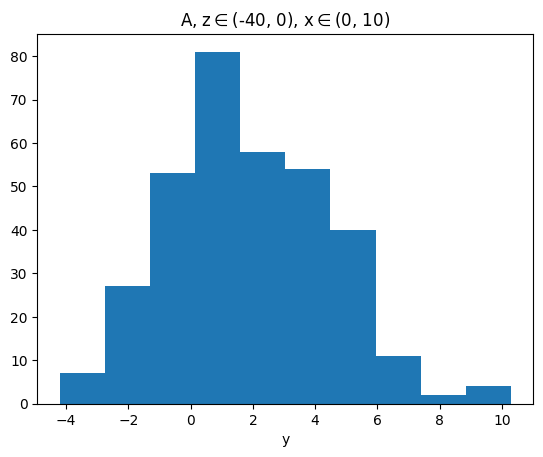
data.plots(
    'hist', cols='y',
    subsets=subset_A,
    global_selection=['z_bins/z(-40-0)', 'x_bins/x(0-10)'], # the intersection of them
    );

Passing different arguments for different subsets

You can pass different arguments to the plot function (i.e., set different options) for each subset that is overplotted on the same axis. This is done using the iter_kwargs argument, as demonstrated in the examples below:

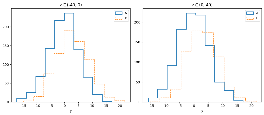
data.plots(
    'hist', cols=['y'], histtype='step',
    plotgroups='class', arraygroups='z_bins',
    iter_kwargs={'linestyle': ['-', '--'], # options for subsets 'A' and 'B' in the 'class' group, respectively
                 'linewidth': [2, 1]},
    )
plt.tight_layout()

data.plots(
    'scatter', 
    cols=('x', 'y'), kwcols={'c': 'x'},
    subsets=('x(-10-0)', 'x(10-20)'),
    iter_kwargs={
        's': [10, 2],
        'marker': ['v', '^'],
        },
    );

[subset] Found subset 'x(-10-0)' in group 'x_bins'.
[subset] Found subset 'x(10-20)' in group 'x_bins'.

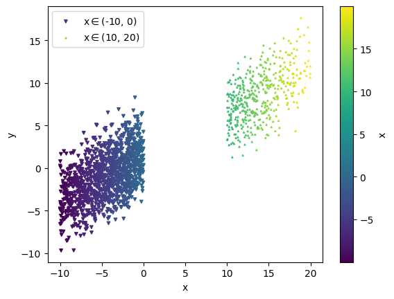
As demonstrated in the example above, when using the built-in scatter plot function, different subsets overplotted on the same axis share the same colorbar, making their color coding comparable.